Dear Reader,

VQE (Variational Quantum Eigensolver) and QAOA (Quantum Approximate Optimization Algorithm) are the two most significant near term quantum algorithms of this decade. If you’re interested in this field you might have come across these terms, along with “variational algorithms” or “hybrid quantum-classical algorithms”.

This will be the first blogpost from a series aimed at helping you understand some of the intricacies of VQE and QAOA and demystifying how variational quantum algorithms work.

This is the whole series:

1. VQE — how it works (this is the one you’re reading)
2. QAOA — how it works
3. VQAs - how do they work
4. VQAs – challenges and progress
5. VQE — challenges and progress
6. QAOA — challenges and progress

The “How it works” parts will describe some of the fundamental ideas behind the algorithms and “Challenges and progress” will discuss the progress and improvements on the basic versions of the algorithms along with some main challenges researchers still face.

You can also find a PDF-version of the whole series on arXiv if that’s the form you prefer.

We will see how it all works out in practice ;) For today’s article, let’s focus on the following topics:

1. What does VQE even do and why do we care?
2. The variational principle
3. What the hell is an “ansatz”?
4. What does the circuit look like?
5. What’s this hybrid approach?
6. Why is it appropriate for NISQ?
7. Example

If you’re not familiar with the term, NISQ stands for “Noisy Intermediate-Scale Quantum”, so roughly speaking means near-term quantum devices.

What does VQE even do and why do we care?

Without going too much into the details and math, I would like to explain what we can use VQE for and why it’s important.

What VQE does

VQE allows us to find an upper bound of the lowest eigenvalue of a given Hamiltonian.

Let’s break it down:

• Upper bound — let’s say we have some quantity and we don’t know its value. For the sake of the example, let’s say it’s the level of water in a well. We know that the water surface can’t be above the edge of the well — if that was the case, the water would spill. So this is our upper bound. We also know that the level cannot fall below the bottom of the well — this is our lower bound. Sometimes when we describe a physical system, it’s very hard to find the real value, but knowing the lower or upper bound can help us estimate what the value might be.
• Hamiltonian — the Hamiltonian is a matrix which describes the possible energies of a physical system. If we know the Hamiltonian, we can calculate the behaviour of the system, learn what the physical states of the system are etc. It’s a central piece of quantum mechanics.
• Eigenvalue — a given physical system can be in various states. Each state has a corresponding energy. These states are described by the eigenvectors and their energies are equal to the corresponding eigenvalues. In particular, the lowest eigenvalue corresponds to the ground state energy.
• Ground state — this is the state of the system with the lowest energy, which means it’s the “most natural” state — i.e. a given system always tend to get there, and if it is in the ground state and is left alone, it will stay there forever.

These “physical systems” and “states” may sound abstract, so let’s try an example that’s a little bit more down-to-earth. I cannot think of anything simpler than a hydrogen atom.

So we have a two-particle system with a proton in the center and one electron. We can describe it with a Hamiltonian. The ground state of the electron is its first orbital. In this configuration it has some energy which corresponds to the lowest eigenvalue of the Hamiltonian. If we hit it with a photon with specific energy, it can get to the excited state (any state that’s not the ground state) — described by another eigenvector and eigenvalue.

With all that in mind, we can reformulate our statement about VQE:

VQE can help us to estimate* the energy of the ground state of a given quantum mechanical system**.

With the following caveats:

* — estimate by providing us an upper bound

** — if we know the Hamiltonian of this system

To be mathematically exact: upper/lower bounds are defined for sets, not single values. So whenever I mention “upper bound of a value” I really mean “upper bound of the one-element set containing given value”. Also, I know that stating “Hamiltonian is a matrix” might be viewed as oversimplification, but I find it a very helpful oversimplification.

Now it’s time to get to the second, arguably more important part:

Why do we care?

There are at least two reasons why we care about using a quantum computers to get the energy of a ground state:

1. Knowing a ground state is useful
2. It’s really difficult to obtain it using a classical computer

Ground state energy is fundamental in quantum chemistry. We use this value to calculate a number of other, more interesting properties of molecules, like their reaction rates, binding strengths or molecular pathways (the different ways in which a chemical reaction can occur). Many of these calculations involve several steps, so an error in the first step will introduce an error to all the subsequent steps. Therefore if one of the values we use in the first step (e.g. energy of the ground state) is closer to the reality, so will be our final result.

The variational principle

In this and the following sections I will go into more technical details of why and how VQE actually works.

The first piece is the variational principle.

Let’s say we have a Hamiltonian \(H\) with eigenstates and associated eigenvalues . Then the following relation holds:

\[H | \psi_{\lambda} \rangle = \lambda | \psi_{\lambda} \rangle\]

which is basically a characteristic equation (eigenequation) for \(H\).

The problem is that we usually don’t know what the eigenstate \(| \psi_{\lambda} \rangle\) is and what’s the value of the \(\lambda\) . So how can we get some estimate of that?

Well, to get the energy value for given state \(| \psi \rangle\), we can use following expression:

\[\langle \psi | H | \psi \rangle = E( \psi )\]

(We usually refer to it as calculating the “expectation value” of \(H\))

If we use an eigenstate we get:

\[\langle \psi_{\lambda} | H | \psi_{\lambda} \rangle = E_{\lambda}\]

For the eigenstate associated with the smallest eigenvalue we would get \(E_0\) (ground state energy). It’s by definition the lowest value we can get, so if we take an arbitrary state \(| \psi \rangle\) with an associated energy \(E_\psi\) , we know that \(E_\psi\) >= \(E_0\) . We get equality if we’re lucky enough that our state is equal to the ground state.

The method described here is known as variational method and the following relation is known as the variational principle:

\[\langle \psi | H | \psi \rangle >= E_0\]

Our \(E_\psi\) is an upper bound for the ground state energy, so exactly what we wanted. The problem is that just knowing any upper bound doesn’t yield much benefit. The closer the upper bound is to the real value, the better. In principle, we could simply try all the possible states and pick the one with the lowest energy. However, this approach isn’t very practical - there are way too many states to accomplish that in a reasonable amount of time. Also, most of the states will give you really bad answers, so there is no point intrying them out.

This is where the ansatz takes the stage!

I know I’ve done a couple of shortcuts here to keep it shorter and easier to digest. If you want to get a formal proof for the variational principle, it’s described pretty well on wiki.

What the hell is an ansatz?

Once you start reading papers about VQE or QAOA, you’ll start noticing that people care a lot about ansatzes. I have missed the definition of ansatz when I started learning, which meant that for a long time it was something rather abstract to me, so here I will try to give you some intuition regarding this topic.

The problem (as mentioned in the previous section) is that we would like to explore the space of all the possible states in a reasonable manner ¹. We do that using parameterizable circuits — i.e. circuits which have gates with some parameters. So let’s take a simple circuit, consisting of a single RY gate as an example. It has a single parameter — rotation angle. With this simple circuit we can represent a whole spectrum of quantum states — namely $\sqrt{\alpha}|0 \rangle + \sqrt{1-\alpha}|1\rangle $ (see picture below).

Below you can find a visualization of this family of states using a Bloch sphere. I’m not going to explain what the Bloch sphere is — if you’re not familiar with it, you can read about it here or elsewhere.

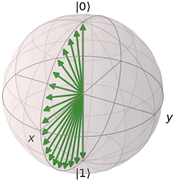
However, there are many states that we can’t represent — e.g. \(1/√2 * ( |0⟩ +i |1⟩)\). In order to cover this state, we need to introduce another gate, e.g. RX. And of course find the corresponding angles.

So RX or RX RY are examples of simple ansatzes. The situation gets more complicated when we have to deal with multiple qubits or entanglement. I don’t want to get into details here, I plan to cover that in the second part of this blogpost; there is also this great paper which covers this topic in depth. But in general we want to have an ansatz which:

• Covers many states — ideally, we want it to cover the whole space of possible states.
• Is shallow — the more gates you use, the higher the chance of something going wrong. We’re talking about NISQ after all.
• Doesn’t have too many parameters — the more parameters, the harder it is to optimize.

If the description above doesn’t give you enough intuition of what it’s about, let’s try with the following metaphor.

Imagine you have a robot. This a simple robot with one rigid arm that can rotate around the central point, like in the picture below:

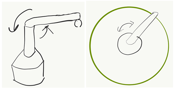
Let’s say the robot has a pen and it can draw. In this case, no matter how hard you try, the most you can get out of it is a circle. How to improve it?

Well, you can add another rotating arm at the end of the first one. Now you can cover much more — a big circle empty in the middle.

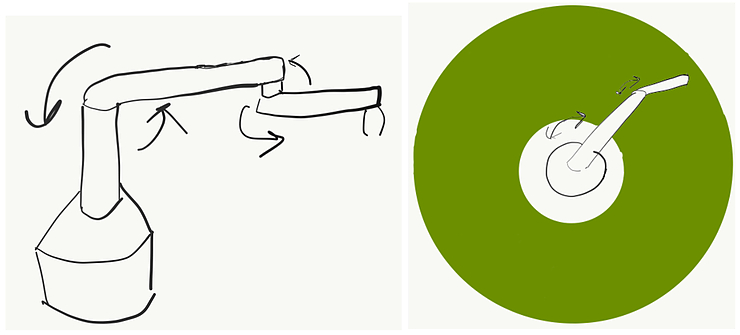
Ok, and what if I told you that actually the arms can only move in a discrete way — i.e. they always rotate by a fixed angle. If it’s small, then you can still cover most of the space. If not — well, you will get a nice pattern. Anyway, it might be beneficial to add additional arms in this imperfect scenario to cover the space better.

Why don’t you add another 20 arms? It sounds impractical for several reasons. The more arms you add, the harder it is to construct and control them, and it’s more error-prone. By the way, you can check out this video to see how crazy you could get with a similar setup in theory. Imagine what these drawings would look like if you got even a 0.1% error in the angles for each arm.

So what does it have to do with our ansatzes? Having a good robot setup will allow you to cover a lot of space and at the same time it would be relatively simple. The same is true for ansatzes. A good ansatz is one that allows you to cover many states and which has a reasonable number of parameters — so it’s easier to control and optimize.

What does the circuit look like?

While writing this section I realized it requires explaining some additional concepts. If it seems difficult, don’t worry — you don’t need to understand it fully to get the big picture. If this is too much at once, you can always come back later.

As we all know, to do quantum computing we use quantum circuits. So what does one for VQE looks like?

It consists of three parts:

• Ansatz
• Hamiltonian
• Measurement

We know what the ansatz part is about — it prepares the state we need in order to apply variational principle.

Hamiltonian — there is a limitation on what Hamiltonians we can use with VQE. We need Hamiltonians constructed as a sum of Pauli operators (X, Y, Z) and their tensor products. So for example we can have the following Hamiltonian: \(XY + YZ + Z\). Or for the multi-qubit case: \(X_1 \otimes X_2 \otimes Y_1 - Z_1 \otimes X_2 + Z_1\).

What might be surprising is the fact that we don’t actually put any of the corresponding X, Y, Z gates into the circuit. We use them to choose in which basis we want to do a measurement.

Most (if not all) contemporary quantum computers perform measurements in the so-called “computational basis”. What it means is that they will tell you whether your state turned out to be 0 or 1. However, that’s not the only way to go. What if we wanted to distinguish between states \(|+⟩ = |0⟩ + |1⟩\) and \(|-⟩ =|0⟩ - |1⟩\) ?

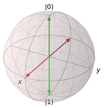
Well, measuring in the computational basis you’ll get 0 and 1 with the same probabilities for both of them, so they’re indistinguishable. To see what might help we can use the Bloch sphere again. Let’s visualize both pairs of states: \(|0⟩\) and \(|1⟩\) (red) and \(|+⟩\) and \(|-⟩\) (green)

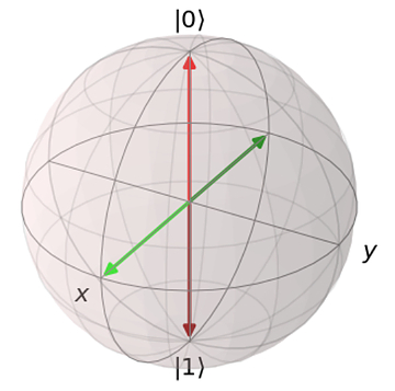
As you can see, in both cases they are on the opposite ends of the sphere. It means that we can switch between them by performing a rotation around the Y axis by 90 degrees.

This gives us a tool to distinguish between \(|+⟩\) and \(|-⟩\) states even if we can measure only whether the state is \(|0⟩\) or \(|1⟩\). If we start from \(|+⟩\) and perform \(RY(π/2)\) rotation (rotation around the Y axis by 90 degrees), we will end up in the \(|1⟩\) state. If we now measure it, we will always get 1. Similar for the other state.

After rotating applying \(RY(π/2)\) to all the states, we will get the following Bloch sphere (notice the colors switched:

Ok, so coming back to our Hamiltonians. The first thing we need to do is divide the sum into its elements, so called “terms”. Now, for each term we look at every Pauli operator and append appropriate rotations to the circuit:

• \(RY(-π/2)\) if it’s X
• \(RX(π/2)\) if it’s Y
• We do nothing if it’s Z

There’s one more caveat here: we actually don’t do it all at once — we create a separate circuit for each term.

And once we’ve done this, we are ready to perform the measurements. But how exactly do these measurements relate to the variational principle we’ve mentioned earlier? Remember this equation: \(\langle \psi | H | \psi \rangle = E_{\psi}\) ?

\(| \psi \rangle\) is the state created by the ansatz. Hamiltonian is composed of sums of Pauli terms, so we can separate it into individual terms and deal with them one at the time: \(H = H_1 + H_2 + … + H_n\).

The question at hand is how to get from here to \(\langle \psi | H_i | \psi \rangle\). We can utilise the fact that \(\langle \psi | H_i | \psi \rangle\) represents the expected value of \(H_i\), which can be approximated by observing (measuring) the state \(| \psi \rangle\) using the right basis (one corresponding to the eigenvalues of \(H_i\)) and averaging the results. The more times we do that, the better precision we’ll get.

One more thing about the averaging - when we do a measurement we get either 0 or 1. Taking all the 0s and 1s and averaging them would give us an expectation value of the measurements, not expectation value of the Z operator. If we look at the Z operator, we see that it has two eigenstates \(| 0 \rangle\) and \(|1 \rangle\) associated with eigenvalues 1 and -1 accordingly. To calculate \(\langle \psi | Z | \psi \rangle\), we need to measure our circuit many times and then substitute every “0” with “1” and every “1” with “-1”.

For more details and some helpful derivations I recommend reading chapter 4 of “Quantum Computing for Computer Scientists” by N. Yanofsky and M. Mannucci.

Ok, so let’s take a look at the following example.

Let’s say the Hamiltonian is: H = 2*Z + X + I (there’s only one qubit, so I’m omitting indices). It is represented by the following matrix:

\[\begin{bmatrix} 3 & 1 \\ 1 & -1\\ \end{bmatrix}\]

We would like to learn its ground state using VQE.

To begin with — we need to choose our ansatz. We don’t want to overcomplicate it, let’s say our ansatz will be \(RY(\theta)\). This will allow us to explore the states \(\cos(\theta) | 0 \rangle + \sin(\theta) | 1 \rangle\).

Our Hamiltonian has three parts : \(H_1 = 2*Z, H_2 = X, H_3 = I\).

The first part is fairly simple. As you recall, if we have a Z gate, we don’t need to add any rotation. So our circuit for the first part of the Hamiltonian will consist just of the ansatz.

You might wonder what should we do with the “2” in front of Z? Well, we will treat it just as weight — after we do measurements and we will be calculating the energy, the results coming from \(H_1\) will count twice as much as the results coming from \(H_2\) or \(H_3\).

In case of \(H_2\) we have one gate: X. So we simply nee to add a \(RY(-\pi/2)\) gate to our circuit.

\(H_3\) is the easiest one of all of them — it’s just a constant factor we need to add to our calculations and we don’t need to do any measurements.

So in this example we need two circuits to use our VQE, you can see them below:

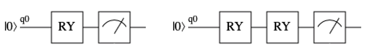
First RYs are ansatzes, and they are parametrized by theta. Second RY in the right picture is actually \(RY(-\pi/2)\). The last symbol is how we depict measurement in quantum circuits.

Our Hamiltonian was: \(H = H_1 + H_2 + H_3 = 2*Z + X + I\)

So if \(\theta = 0\), then we will get 2 for \(H_1\), 0 for \(H_2\) and 1 for \(H_3\). So our \(\langle \psi(0) | H | \psi(0) \rangle = 3\).

If \(\theta=\pi\), we get 2*(-1) for \(H_1\), 0 for \(H_2\) and 1 for \(H_3\), \(\langle \psi(\pi) | H | \psi(\pi) \rangle = -1\).

Going through all the possible values of \(\theta\) would be cumbersome, so I will tell you how approach the problem of finding a good value of theta in the next section.

This example was pretty simple and you might wonder: “Ok, but how do I deal with the case, when there are more than one Pauli matrices in one term?”. It turns out that whenever you start multiplying Pauli matrices, in the end you always get another Pauli matrix multiplied by some constant. So you can always simplify your term in such way, that you will end up with a single Pauli matrix.

And what if I have more qubits? Again, we treat each term separately, perform all the rotations that we need at the end and measure all the qubits that we need.

If you would like to calculate these by hand, you might find the notes by Christoph Trybek helpful.

Hybrid approach

As mentioned earlier, VQE is a hybrid, quantum-classical algorithm. It means that we don’t perform all the computations on a quantum computer, we use a classical one too. So what does that look like?

You remember that ansatz has a lot of parameters, right? The problem is that we don’t know which parameters are good and which ones are crappy. So, how do we learn that? Well, we treat it as a regular optimization problem.

Usually we start from a random set of parameters — which corresponds to a random state (keep in mind it’s created using the ansatz that we use — so it’s not a “random state chosen from the set of all possible states”, but a “random state chosen from the set of all possible states we can get with given ansatz”). We perform measurements, so we know the corresponding energy (we also use the term “expectation value”).

Then we slightly change the parameters, which corresponds to a slightly changed state. After we perform measurements, we should get a different energy value.

If the new energy value is lower, it means that we’re moving into a good direction. So in the next iteration we will further increase those parameters that have increased and decrease those that have decreased. If the new energy value is higher, it means we need to do the opposite. Hopefully after repeating this procedure many times, we will get to a place where no matter what changes we do to the parameters, we can’t get any better — this is our minimum.

The optimization strategy I described is pretty trivial and it’s good only as an example. Choosing a right optimization method for your problem might decide whether you’ll succeed or not and is pretty difficult — there are no silver bullets here. You can choose from a range of methods, like SGD (Stochastic Gradient Descent), BFGS or Nelder-Mead method.

Ok, but this section was supposed to be about explaining how the hybrid quantum-classical thing works, right?

So the idea is that we use a quantum computer (sometimes called QPU — quantum processing unit) for one thing only — to get the energy value for a given set of parameters. Everything else — so the whole optimization part — happens on a regular computer.

To make it more tangible here’s a (probably incomplete) list.

What a QPU does:

• Given a set of parameters, returns us a set of measurements.

What a classical computer does:

• Given a set of measurements calculates the energy value (it’s usually some kind of averaging)
• Performs optimization procedure
• Calculates what a new set of parameters should be
• Checks whether we have reached the minimum
• Makes sure we don’t make more iterations than we should have done

Why is this appropriate for NISQ devices?

As already mentioned, NISQ stands for “Noisy Intermediate Scale Quantum” (John Preskill explains what it exactly means in this video or paper) — so not perfect million-qubit devices that are needed to run the famous Shor’s or Grover’s algorithms, but rather several-qubit prototypes.

Some of the main disadvantages of NISQ devices are:

• There’s a lot of noise — e.g. every time you apply a gate, there’s some substantial chance (e.g. 0.1%) that you’ll actually apply a different gate. And this is just one of many flavours of noise you can get.
• The qubits don’t live for too long — after some time you can be pretty confident that whatever information was stored in your system, it’s lost. So the number of operations you can perform in this time is limited.
• You don’t have too many qubits — right now (late 2019) the biggest chips have around 50. Also, there might be some restrictions on which qubits can interact with each other.

This translates to a pretty clear set of restrictions on your quantum circuit:

• You can use only N operations per qubit (so called “circuit depth”)
• You can’t assume everything will go according to plan and there will be no errors along the way. Even if there are errors, you should still get a reasonable (though not perfect) answer. We call this “robustness”.
• Obviously, you can’t use more qubits than you have.

So why exactly VQE is a sensible proposition for NISQ devices?

1. It’s pretty flexible when it comes to the circuit depth, so you can make some tradeoffs. You can use a pretty simple ansatz if you want to keep your circuit very shallow. But once you have a machine which allows you for a deeper circuit — you can use more sophisticated ansatzes and your performance might increase as a result.
2. VQE has been shown to be somewhat resistant to noise — i.e. even in the presence of noise (up to some levels) it gives you the correct results. Some even claim that a pinch of noise might help with the optimization process, because it helps to escape local minima.
3. There are some practical problems that do not require a lot of qubits. One example can be nitrogen fixation - an important industrial process (Honestly, it’s not directly about VQE, but you can read details in this paper).

Example

If you would like to know how the VQE works, here is a link to a jupyter notebook with an example in pyQuil.

It’s not sophisticated, but it follows exactly the steps you have seen here already. I encourage you to play with it, see how it works, try to improve it. Write your own, proper version of VQE and check if it gives you the same results as different open source implementations.

And if you do - make sure you let me know!

Edit (23rd December 2019): Davit Khachatryan has written an excellent tutorial for VQE - it’s much more detailed than my example and also gives an example of a two-qubit circuit. You can find it here. I strongly recommend it!

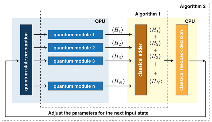
Also, I think now you have finally all the pieces to appreciate the following picture from the original VQE paper. It shows the overview of the whole algorithm and I think it might be helpful in understanding how all different elements come together.

You can read “Quantum state preparation” as “ansatz” and “quantum module” as “adding rotations to enable measurements in the right basis”.

Closing notes

I hope you’ve enjoyed this blogpost. It was more technical than my usual writing so please let me know if you found it useful in any way and if you would like to see more of that. Honestly, I was tempted to go much much deeper into the math here, but then this would end up being twice as long — but for the curious readers out there, I really recommend digging deeper; I provided some resources in the text.

If you have any feedback or some points have been unclear — please let me know!

Huge thanks to everyone who contributed to this blogpost, especially:

• Rafał Ociepa
• Ntwali Bashige
• Peter Johnson
• AJ Roeth
• Sukin Sim
• Tanisha Bassan
• Tomasz Sabała
• Davit Khachatryan (for spotting errors in my math!)

Also, thanks to the quantum-circuit and qutip teams for creating great tools I used for drawing circuits and Bloch spheres (accordingly).

If you don’t want to miss another blogpost for me, please sign up for the newsletter. And if you liked this one, I’m sure you’ll like the other parts of the series - for links look at the top of this post!

Have a nice day!

Michał

Footnotes:

---

• All Posts (28) ,
• Quantum computing (19) ,
• Algorithms (6)