
Dear Reader,
Today we will delve into the details of QAOA – variational quantum algorithm for solving combinatorial optimization problems.
We already covered a lot in previous articles in this series, so I highly recommend going through that first, especially articles 2, 3 and 4, as they are all very relevant.
- VQE — how it works
- QAOA — how it works
- VQAs - how do they work
- VQAs – challenges and progress
- VQE — challenges and progress
- QAOA — challenges and progress (this is the one you’re reading)
Update: about a month after writing this a review paper on the topic came out by Blekos et al.. I don’t refer to it in the blogpost, but it covers many of the variants of QAOA and is much more comprehensive than this blogpost could ever be! I recommend reading it to anyone interested!
QAOA vs QAOA
Before we even get into a detailed discussion about the algorithm itself, let’s first talk about naming. The original QAOA algorithm presented by Farhi et al. is called Quantum Approximate Optimization Algorithm. However, in 2018 Stuart Hadfield et al. presented a more general algorithm which is called Quantum Alternating Operator Ansatz. Which also spells “QAOA”. You might have a couple of questions now:
- Why would they do that?
- What’s the difference between these two?
- If I hear “QAOA” what exactly do people mean by it?
Let me quote the Hadfield’s paper:
We reworked the original acronym so that “QAOA” continues to apply to both prior work and future work to be done in this more general framework. More generally, the reworked acronym refers to a set of states representable in a certain form, and so can be used without confusion in contexts other than approximate optimization, e.g., exact optimization and sampling.
This means that “the original QAOA” is just a subset of “a more general QAOA”. One of the differences is that in the original QAOA the Hamiltonians which we use are defined in a specific way, while the more general framework allows for much more flexibility. Plus the more general framework is not designed specifically for “approximate optimization” but also for other uses.
So if you hear “QAOA” which one people mean? Well, I’d argue that most of the time people mean the “more general QAOA”, even if they don’t necessarily realize that or what’s the actual difference. I think that most of the time if someone means “original QAOA” specifically they refer to it as “vanilla QAOA”, “basic QAOA”, “Farhi’s QAOA” or something similar.
Problem-related issues
There are three topics I wanted to talk about, which are more about the problems we’re trying to solve rather than the QAOA algorithm itself. Dealing with these challenges is important for any algorithm which tries to solve optimization problems, quantum or classical. Some are more apparent in one class of algorithms, some in others, but over the years I learned that they all can heavily influence the results of your optimization routine, so I think it’s worth discussing them here.
These are:
- Problem formulation
- Constraints
- Problem encoding
Problem formulation
In general, when you try to solve optimization problems, there is a huge payoff for understanding your problem better and coming up with a better formulation. By formulation I mean understanding the real-world problem and expressing it in a way that an algorithm can solve and maybe adding some problem-specific improvements to the algorithm. This is in opposition to coming up with a better optimization method for a given class of problems, fine tuning it, etc.
Let’s take a look at the following problem – you are in charge of IT infrastructure at a campus. You have a team of 5 people and you have to service equipment in various buildings at the campus. Every day you get calls from people around the campus about the issues that your team needs to solve. For each request you:
- identify where the issue happened
- estimate how long it will take to solve it.
The problem is how to assign your team in an optimal way?
One approach would be to model this as Capacitated Vehicle Routing Problem (CVRP, it’s a more complicated variant of Traveling Salesman Problem).
In such formulation you can say that:
- The capacity of each person is 6 hours per day
- Each person shouldn’t spend more than 1 hour driving around the campus, which translates into a constraint that the route itself needs to be under 1 hour.
- You are fine with not solving all the requests every day (i.e. not visiting all the cities)
You also decide that your cost function is the number of issues you can solve per day.
Do you think it’s a good formulation?
Well, it depends. Below you can find a couple of questions that one needs to ask in order to model this specific problem better:
- Are all the people on the team equally skilled? If one of them is new to the job and another one is a veteran, you should probably start expressing the time estimates differently, e.g. depending on one’s experience or in abstract “points” rather than time. In the latter case, the expert person would have higher capacity.
- How accurate are your time estimates for solving those problems? If they’re not very accurate, the mathematical model might have a huge mismatch with reality. If they’re not very accurate, can you model how inaccurate they are, perhaps using a normal distribution?
- How much time does it take to travel between different buildings on campus? If there are 3 buildings which are all 5 minutes apart, perhaps it’s worth modeling them as one node – that would decrease the complexity of the graph. If getting from one building to another takes less than 10 minutes, perhaps it’s negligible and you would be better off modeling it as a scheduling problem and not CVRP?
- Do issues have different importance?
- Given that your cost function depends on the number of problem solved per day, it might lead to a situation where one 6-hour long problem never gets scheduled, because there are always multiple 1-hour problems popping everywhere. Is that acceptable?
- Can some problems be solved remotely? If so, how would you model that?
- What if a particular problem takes more than a day to solve?
I hope that’s enough to make this point, perhaps the most important from the whole blogpost:
You can have the absolutely best algorithm for solving combinatorial optimization problems, but in the end, if your problem model doesn’t match reality well, who cares?
Constraints
Imagine you have a store and you sell two products: X and Y. You want to maximize the profits from selling them. Profit equals revenue minus cost:
P=R−CRevenue is equal to the amount of X sold times its price and same for Y.
R=pxx+pyyThe costs are trickier, as the more products you have, the pricier it is to store it:
C=cxx2+cyy2.
Your goal is to order the optimal amount of X and Y so that you can maximize your profit.
Well – that’s a simple quadratic function. You can solve it analytically or just use a simple gradient descent optimizer and find it in no time. But let’s add some constraints to make it more realistic. Let’s say you have a limited capacity of your storage, so:
0<x+y<C1Also, they shouldn’t be negative: x>=0 and y>=0.
On top of that, your supplier tells you that process for creating X and Y is correlated and you can’t just buy only X or only Y, but there’s also some upper cap on their production in relation to each other, so you need to add the following constraint:
C2<=x∗y<=C3Oh, and on top of that, X is sold in discrete quantities (x is an integer), but Y is a liquid so you can buy any quantities (y is a real number).
Well, now our problem is much more interesting and it’s not immediately obvious how to solve it. As you might guess, people came up with some techniques to deal with such constraints. Unfortunately not all of these methods are applicable to all types of cost functions, all types of constraints or all types of optimizers. As it’s quite a broad topic, here I’ll focus only on two methods that you might encounter in QAOA-related literature problems.
First of them works by using something called a “penalty function”. It is a way of modifying your cost function, by introducing some artificial terms which would “penalize” if the variables don’t meet the constraint. Let’s use our favorite MaxCut. As you might recall from previous parts, the cost function of MaxCut is:
C=∑(i,j)∈Ewij(1−xixj),
where E is a set of all the edges in the graph.
But what if we had a constraint that one group needs to consist of exactly 5 elements? How could we express it mathematically? Since xi is either 0 or 1, we can arbitrarily say that we want the group represented by ones to have exactly 5 elements. In such a case we know that ∑xi=5. We can also rewrite it as: 5−∑xii=0. How do we incorporate this in our cost function? Well, here’s the trick. We transform it into the following term:
P=P1(5−∑xi)2and then just add it to the cost function:
Cnew=C+PSince we want to minimize the value of Cnew, any solution x which doesn’t meet the constraint will make the value of Cnew higher, so it will be a worse solution. Since P1 is an arbitrary constant which doesn’t have any real-world meaning, we can select it to be arbitrarily high. E.g. if our values C are usually in the range of 0-10, we can set P1=100, so that any minor violation of the constraint would result in an extremely high penalty to the cost1. Basically what we did is we transformed a constrained problem (cost function C and our constraint) into an unconstrained one (just cost_function Cnew without any constraints).
This method has some pros and cons – it’s relatively simple and it works for basically any problem, as you can always modify your cost function. However, it doesn’t work well with all types of optimization methods and is a little bit more tricky to use with inequality constraints (i.e. ≥,≤). You can find examples of this being incorporated into the cost function in everyone’s favorite “Ising formulations of many NP problems” by Andrew Lucas, see e.g.: section 7.1 . Another example of how to do that is in section 3.1 of this paper (again by Stuart Hadfield)2.
There is another way to avoid getting solutions you don’t want, and it works particularly well with problems where solutions have some inherent structure, as is the case for many combinatorial optimization problems. Let’s take the Traveling Salesman Problem (TSP) as an example3. For 5 cities the solution can look like this: [5, 2, 3, 1, 4], which specifies in what order we visit cities. An incorrect solution might look like this: [5, 2, 3, 1, 2] – as you can see we’re visiting city 2 twice in this case, but we’re missing city 4, which violates the constraints.
How can we ensure our solution is always correct? There are two components to the solution:
- Start from a valid solution (i.e. one doesn’t violate constraints)
- Create new solutions by performing only operations which transform a valid solution into another valid solution.
In the case of TSP such operations would be swapping elements in the list. So we could transform [5, 2, 3, 1, 4] into [4, 2, 3, 1, 5], which is also a valid solution, but with this method we would never get anything like [5, 2, 3, 1, 2].
Easy to do with lists, but how does one do that with quantum states? I talk more about it in the section about alternative QAOA ansatz!
Encoding
Another important topic is how do you encode your problem to fit a particular algorithm. Let’s think about how to describe the TSP problem in a mathematical form and different ways to encode solutions to it.
The most natural (at least for me) way is to define a distance matrix. It is a matrics which tells us what’s a difference between each pair of cities. For three cities it can look like this:
| A | B | C | |
|---|---|---|---|
| A | 0 | 5 | 7 |
| B | 5 | 0 | 10 |
| C | 7 | 10 | 0 |
We know that the distance from A to B is 5km, from B to C is 10km and from A to C is 7km. How would we encode the solution? Simply as: [A, B, C], [B, C, A] etc.
We can easily switch to integer labels (A=>1, B=>2, C=>3), which will make some math down the road easier (like indexing rows and columns of the distance matrix).
Ok, but what if our machine has a limited number of integers it can work with for expressing the solution. In the case of a quantum computer it’s actually just 0 or 1. So how would we encode the solution to our 3-city problem?
Well, there are multiple ways to do this. The simpler one (perhaps) is called “one-hot encoding” or “unary encoding”. In this encoding, we encode each city like this:
- A -> 100
- B -> 010
- C -> 001
Now if we want to represent a route: A -> C -> B, we can write it as “100 001 010”. Each bistring will consist of three blocks, each represent one moment in time. And then each block will consist of three bits, each representing a city. So in this case having “001” in the middle means, that we visit city “C” in the second time step. This allows us to easily encode constraints, such as “you can be only in one city at the time”, as you just need to check if any given block contains only a single 1.
However, one thing people often say when looking at the unary encoding is that it’s very space inefficient. Indeed, it will take you n2 bits to encode a solution for the problem with n cities. So perhaps we could use binary encoding. In this case we will have:
- A -> 00
- B -> 01
- C -> 10
Now, we use only 6 bits to encode the solution and it actually scales as $n \cdot log(n)$, which is pretty good!
There are, however, a couple of issues here. First, the bitstring “11” is undefined. You can write a route containing it, but it doesn’t mean anything. One way to deal with it is to add a constraint that will prohibit its occurrences, but it adds more complexity. Second, encoding the “basic constraints” of the problem, like “each city needs to be visited only once” is more involved than in the previous case.
There’s plenty of trade-offs when it comes to choosing encoding, and you can come up with many different variants (or even combining multiple encoding at the same time). I won’t get into any details, but if you are interested, I recommend reading this paper by Nicholas Sawaya et al.
We didn’t even discuss how those encodings impact the construction of the cost Hamiltonian for our problem, as it would be rather tedious. I just wanted to signal this as another important decision which you need to think about when you try to solve optimization problems, especially with quantum computers.
Parameter concentration
Ok, now we’re done with those “general optimization topics”, let’s get into some QAOA-specific topics. Let’s start with a very interesting phenomenon first described by Brandao et al. Consider a class of problems: MaxCut on 3-regular graphs4. Let’s take one problem instance (i.e. one specific graph) and find good parameters for it. And now let’s take 100 other graphs of the same size and see how well these parameters would do?
It turns out that good parameters for one instance work very well on 100 other similar instances of the same size. But that’s not everything – they also work very well on graphs of different sizes, but of the same type. So for example a graph with 10 nodes and the other one with 20 nodes. Also, good parameters work equally well and bad parameters work equally badly. This inspired us to do a little bit of investigation with the visualization package we developed at Zapata, orqviz. As you can see in the plots below, for several graphs from the same family which differ in size, the cost landscapes look very similar around the same parameters. I’m skimming over a lot of details here, see the paper for details.
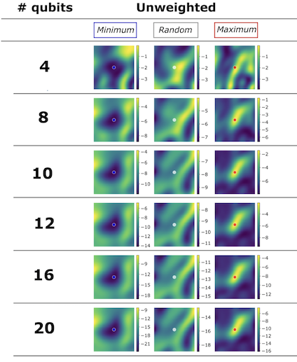
It’s pretty crazy if you think about it – we can take one graph, find good parameters for QAOA and just use them for another graph and it just works. For now this has been investigated only for simple types of problems and I don’t think this will hold for much bigger real-world problems, but it’s still an extremely interesting phenomenon to investigate. I think this paper by Jonathan Wurtz gives some insight on what might be going on, especially for 3-regular graphs.
Modified cost functions
In many VQAs we are interested in calculating the expectation value of a particular operator. This is a very reasonable thing to do if the expectation value is what we’re looking after. While using QAOA the expectation value corresponds to the value of the cost function. However, we don’t really care about the value of the cost function. Sure, it would be nice to get to the minimum, but its numerical value is usually not what we’re after. What we are after is the solution of our problem which gives us this low cost function value.
Before we go further let’s revisit a basic question: how do we use quantum computers to calculate the expectation value?
- We run a particular circuit and obtain a bitstring.
- We use this bitstring to calculate the energy value based on some Hamiltonian.
- And since quantum computers are probabilistic, we need to run it N times to get good statistics.
Now let’s imagine that we have an ansatz and two sets of parameters. Here are two tables, one shows the energy of each bistring and the other one the measurements we get when we run the circuits with those two sets of params:
| Energy | |
|---|---|
| bitstring_1 | 10 |
| bitstring_2 | 1 |
| bitstring_3 | 0 |
| bitstring_4 | 1000 |
| bitstring_1 | bitstring_2 | bitstring_3 | bitstring_4 | expectation value | |
|---|---|---|---|---|---|
| params_1 | 900 | 100 | 0 | 0 | 9.1 |
| params_2 | 0 | 0 | 900 | 100 | 900 |
Which set of params is better?
Well, if we just look at the expectation value, the first one is much better. But if we also look at the quality of the bitstrings we obtained – that’s a different story. Second set of parameters gives us bitstring_3. And bitstring_3 has the lowest energy value from all the bitstrings we’ve seen for this problem – perhaps it’s even the best possible solution to our problem? And, as we mentioned, in the optimization problems we are more interested in obtaining the best possible solution to our problem, rather than obtaining the best expectation value.
The phenomenon we see here is a result of superposition. In the case of Ising Hamiltonians representing combinatorial optimization problems, there is a quantum state which gives you a particular bitstring (representing your solution) with 100% probability. But since we have superposition, we can have states which represent more than one solution at once (as seen above). This results in this somewhat unintuitive situation, where we have a state with higher expectation value which provides a much better solution than another state with lower expectation value. Can we do something about it? Sure we can!
What if we simply discarded 50% percent of measurements with the highest cost value? This is how our table would look like:
| bitstring_1 | bitstring_2 | bitstring_3 | bitstring_4 | expectation value | |
|---|---|---|---|---|---|
| params_1 | 400 | 100 | 0 | 0 | 8.2 |
| params_2 | 0 | 0 | 500 | 0 | 0 |
This technique is called CVaR and has been proposed by Barkoutsos et al.. It can also be applied to other VQAs, I recommend checking out the paper as it’s a really good read. Results in this follow-up work suggests that CVaR is a must-have tool in anyone’s QAOA’s toolbox.
It’s worth mentioning that apart from CVaR, there is another method which works similarly, called “Gibbs Objective Function”. In this case the cost function is defined as:
By using such a cost function instead of a standard one, we increase the weight of the low-energy samples. The original paper by Li et al. provides a good intuition about how and why it works, so if you’re interested, I recommend reading section III of it.
Other ansatzes
One of the fundamental building blocks of VQAs is ansatz. We discussed its importance in detail in the post about VQAs and what are some considerations in using one versus another.
In the first QAOA post we have described the most basic version of the ansatz for QAOA, let’s do a quick recap here.
QAOA ansatz is generated by two Hamiltonians, summarized by the following table:
| HB | HC |
|---|---|
| Associated with the angle beta | Associated with the angle gamma |
| Independent of the cost function | Is defined by the cost function |
| Called “Mixing Hamiltonian” | Called “Cost Hamiltonian” |
QAOA creates the state: |γ,β⟩=U(HB,βp)U(HC,γp)…U(HB,β1)U(HC,γ1)|s⟩, where U(HB,β)=e−iβHB and U(HC,γ)=e−iγHC and |s⟩ is the starting state.
There can be a lot of variation in how you construct the circuit within this framework, here I will go through two of them: Warm-start QAOA ansatz and Hadfield’s QAOA.
These are by no means the best possible ansatzes, but I think they show well how one can approach constructing new ansatzes.
Warm-start QAOA
In optimization we have a concept of “warm-starting” the optimization process. It happens when we use information from previous optimization runs to start with some reasonable initial parameters. In QAOA we can use some classical optimization process to get some reasonable solutions. Then we can inject this information into our ansatz, which hopefully will work better now. How does it work in practice?
Let’s say we have a problem, for which the solution is a binary string, and a classical solver which can solve a “relaxed version” of this problem. “Relaxation” here means that instead of limiting ourselves to integers, our solution can contain any real number between 0 and 1. This is reasonable, as often continuous versions of a problem are simpler to solve than discrete ones. We denote our classical solution as |c|∗ and based on this we construct a vector θ for which every i-th element is defined as: θi=2arcsin(√c∗i). Now for the initial state we use state, where each qubit is set to |i⟩=RY(θi)|0⟩. In this state the probability to measure given qubit in state |1⟩ is equal to c∗i. On top of that, we also modify the mixing Hamiltonian to the following form:
HwsM=n−1∑i=0HwsM,iwhere
HwsM,i=−sinθiX−cosθiZand X,Z are Pauli operators. This is easily implementable using RY and RZ gates.
There is a lot more to this, so if you’re interested I recommend Egger et al which shows how this basic idea can be extended and elaborate much more on why these choices have been made. Also, it’s worth noting that there are other approaches to warm-starting QAOA, such as Tate et al (and the follow-up work).
Quantum Alternating Operator Ansatz
This section is about the framework that was proposed by Stuard Hadfield (his thesis and Hadfield et al.). I won’t go into too many technical details about it, as it’s described very well in there, with examples for specific problems and reasoning behind it. Here I would like to just give you a general understanding of how this family of ansatzes work. As initially proposed, it was intended to be used with constrained problems (please read the section about constraints first if you haven’t already).
The main idea is as follows:
- Start from a quantum state which represents a valid solution.
- Use mixing Hamiltonian which allows you to evolve your state only within feasible subspace. Which means it transforms quantum states representing valid solutions into other quantum states representing other valid solutions.
Therefore a circuit here is built from three elements:
- Initial state – we need to start in a state which represents a feasible solution to the problem. Not the optimal one (this would pretty much kill the purpose), but just some which doesn’t violate any constraints. This can also be a superposition of multiple feasible states, which usually gives better results.
- Mixing Hamiltonian – this Hamiltonian is responsible for changing the provided state. So it can be implemented in such a way, that we only allow for the operations that transform feasible states into feasible states. For example in the case of TSP this means having a Hamiltonian which represents list permutation. It also gives a more flexible framework for constructing these operators, as they no longer need to necessarily be exponentials of a single Hamiltonian, as in regular QAOA.
- Cost Hamiltonian – this is our old good cost Hamiltonian, no changes here :)
As I’ve learned in some of my own projects, implementing an ansatz from this class can give you a significant boost in the quality of the results. However, it comes at a price – those circuits are usually deeper than the alternatives. Let’s discuss such tradeoffs in the next section!
Implementation tradeoffs
As we discussed, solving a problem using QAOA requires making several decisions – how to formulate the problem, how to encode it into an Ising Hamiltonian, what ansatz to choose, which cost function to use, etc.
Each of these comes at a certain cost – let’s look at the choice of the ansatz. When we consider different options it seems that Hadfield’s ansatz looks like a decent idea. However, it incurs some extra costs – first, we need to create the initial state. Depending on the particular case, it might be either easy and cheap (in terms of number of required gates) or very non-trivial, especially if we want to create a superposition of many feasible initial states. Another hurdle is implementing the mixing Hamiltonian. The standard “all-X” mixing Hamiltonian can be implemented by a single layer of RZ gates. On the other hand, some of the Hamiltonians proposed in the paper are pretty complicated and implementing them might require creating a circuit with hundreds of gates. Fortunately, the cost Hamiltonian will be the same most of the time.
Let’s say that for the particular problem that we want to solve, the circuit using Hadfield’s ansatz is 10x longer than the basic one. This means that it will run 10x longer. Can this be even worth it? Well, it might turn out that our ansatz gives us the correct answer with 10% probability, while using vanilla ansatz it would be 0.1%. So even though we need 10x more time to run our circuit, we need to run it only 100 times, to get 10 good samples, while with the basic version, we would need to run it 10000 times. Therefore, using a more expensive ansatz would still give us an order of magnitude improvement in the runtime.
Obviously, this is an overly simplified toy example – in the real case the analysis would be much, much more difficult to do – we would need to model how different circuits are susceptible to noise, try to estimate how fast the optimization of the parameters converges in various cases etc. Taking all of those factors and various combinations into account is impossible and requires extensive experimentation to come up with the set of methods that will be appropriate for solving the problem at hand.
However, certain calculations can be done relatively quickly – for example, if we have some theory to back up a claim that a particular method would require getting 1000 more samples than another one, or if one circuit is 1000x longer than the other one, we can probably rule them out, cause it’s unlikely, they will yield enough benefits, given that they already have 3 orders of magnitude longer runtime. Therefore, it’s always good to look critically at the methods we plan to use – even if it’s not possible to get the precise numbers, we might still get some good insight about the tradeoffs.
Parameter initialization
Imagine two people are looking for treasure on an island. One is a 9 years old girl with a broken leg, walking with crutches. The other one is a 30-years old commando who spends two months a year on survival trips to the Amazon jungle. They both have the same map to the treasure and both start the treasure hunt from different places on the map.
Who is more likely to win?
Well, I wouldn’t bet too much on a girl.
However, what if I told you that the girl was lucky enough to start 10 meters away from the treasure chest, while the guy starts on the opposite side of the island, behind 2 rivers and an active volcano?
This changes the picture.
It’s similar to optimization – you will spend much less time looking for optimal parameters if the initial parameters are close to optimal. And starting from a bad place will make things so much harder for you. Since VQAs are all about finding optimal parameters for a given problem, it’s no surprise that people spend a lot of time trying to find a way for good parameter initialization.
Here I will cover a couple of methods for parameter initialization – layer-by-layer optimization (LBL), INTERP and schedules. One thing before we start – even though I call them “parameter initializations” strategies, they are sometimes tightly related to the optimization process.
The simplest one is LBL – here we start from a small number of layers which is easy to optimize due to the small number of parameters. Once we have found optimal params, we keep them, add a new layer, initialize it with random parms and repeat the process. And again, and again until we reach our target number of layers. There are different variants of this approach, but you can see that it’s pretty resource-intensive, as we have to basically run about N optimization loops, where N is the target number of layers.
This has been improved by introducing a method called INTERP. It’s based on the observation that gammas and betas seem to increase monotonically (see fig. 2 from Zhou et al.). Therefore, we don’t have to initialize the new layer randomly – if we have good parameters for layer N-1, we can predict what would be good parameters for N, tune all the params a little bit and repeat the process. This can be done using a straightforward interpolation, but the authors also suggested a more sophisticated method called “FOURIER” – I recommend reading the original paper, it’s extremely interesting. There is also a recent work by Sack et al, which provides some more theoretical background and intuition why and how INTERP works.
Methods like this will work well for a relatively small number of layers, but what if we talk about the future where we could have thousands of layers? It turns out that in this limit we might be able to get decent results by using something called “schedules”. In this paper the authors decided that they’ll choose values for betas and gammas defined by: γ(f)=Δf and β(f)=(1−Δ)f. Here f has values from 0 to 1 and for a case with a total of p layers, we substitute f with fj=jp+1 for a j-th layer. Δ is a free parameter we need to pick ourselves. Therefore schedule is basically a curve from which we take our parameters. This work by Sack and Serbyn also discusses similar ideas.
I like how these methods fit together – we’ve seen in the INTERP paper that the parameters change monotonically, so why not just make a simple assumption that the change is linear and see where it leads us? Since finding optimal parameters is an extremely computationally expensive problem, it would be great if using schedules like this (or more involved) would spare us optimizing parameters or provide us with really good initial params. But to see how this will play out in practice, I think we need to start running more of these on real devices.
Closing notes
There are a lot of other developments in the QAOA space. RQAOA, Multi-angle QAOA and ADAPT-QAOA to name a few. However, if I tried to cover all these topics, this would soon become a review paper and not a blogpost, so I had to stop somewhere :)
I hope you found this blogpost helpful in understanding some more advanced concepts around QAOA and now it will be easier for you to explore these concepts by yourself.
And of course, I wanted to thank to people that helped me with writing this blogpost, namely:
- Matt Kowalsky
- Stuart Hadfield
Since this is the last blogpost in my series about variational quantum algorithms, I just wanted to say that I’m really grateful for all the positive feedback I got from various people who read these articles over the years. When I started writing it 3.5 years ago, I didn’t know it would take me so long to finish it. But here we are! Thank you for joining me on this VQA journey, I learned a lot in the process and I hope you did as well. You can find a PDF-version of the whole series on arXiv.
And if you want to know about other projects I’ll be working on, please subscribe for the newsletter :) I have one cool paper on QAOA coming out very soon and some good content about quantum software.
Have a nice day!
Michał
Footnotes:
-
In practice, tuning the values of the penalties constants might be a significant problem in itself. Too small and it doesn’t serve its function. Too high and it might lead the optimizer to behave in unexpected ways. Not to mention interplay between multiple penalties! ↩
-
It also shows how to map real functions to Ising Hamiltonians – something I didn’t know is possible and find it pretty cool! ↩
-
If you are not familiar with it, you can find an explanation on wiki. ↩
-
3-regular means that each node connects to exactly three other nodes. So each node has exactly 3 neighbours. ↩