
Dear Reader,
This is the fourth part of my series about Variational Quantum Algorithms (VQAs). In previous parts we learned how these algorithms work in theory, now it’s time to learn more about some challenges, current research, and practical considerations about them.
In this article, we’ll focus on the general issues with running VQAs on quantum computers, regardless of their specific structure. We’ll go into more detail about challenges unique (or at least more characteristic) for VQE and QAOA in the next two posts.
If you haven’t read the previous parts or you’re not familiar with these algorithms, here you can find previous parts of this series:
Also, Here’s a list of the concepts that we talked about in previous posts. If you’re not sure what they mean, please stop for a moment to refresh your memory, as I won’t be explaining them here again.
- Ansatz (VQE article, “What the hell is Ansatz?”)
- Hamiltonian (VQE article, “What VQE does”)
- Expectation values (VQE article, “The variational principle”)
- Hyperparameters (VQA article, “Basic setup”)
While writing this article I heavily relied on two excellent review papers: from Alan Aspuru-Guzik group of University of Toronto and a big collaboration of various institutions. You can find a lot more details there!
Let’s begin!
Hardware-related problems
No matter what algorithm you want to run on the NISQ devices, you need to deal with the following issues:
- Noise
- Connectivity
- Size of the device
- Limited gate-set
Noise types
Understanding how noise and error impact quantum computation is an entire subfield known as quantum characterization, verification and validation (QCVV). We’ll stick to just a cursory description of a few important concepts.
On a physical device, two important concepts involving error are:
- Decoherence—unwanted interaction between the qubits and their environment that causes the quantum state of the qubits to lose its purity
- Control error—physical operations (e.g. laser pulses) that are not exactly as intended, causing the actual quantum gates to differ from the target quantum gates
In practice, these are quite intertwined and difficult to separate. Generally, they lead to three types of error in a quantum computation:
- Coherent error—during a quantum circuit the quantum state is shifted to a different quantum state
- Stochastic error—during a quantum circuit the quantum state becomes an average of different quantum states
- Measurement error—you might have a perfect quantum computer with zero noise and then at the end of the circuit, your measurement procedure might assign an incorrect state when you measure it
Coherent and stochastic error differ in how they cause overall error in a quantum circuit to accrue. Coherent error accrues less favorably in that the quantum state can continue to be shifted in the wrong direction. With stochastic error there can be some canceling out of the errors so that on average they leave you close to the intended state.
If you’d like to learn more, see section 8.3 of Nielsen and Chuang. For those looking for a deeper rabbit hole, here are some more papers: Kueng et al., Zhang et al., Bravyi or Geller and Sun.
To give you some ideas about how it looks like on real devices we have today, let’s take a look at the specs of the device from ETH Zurich used in this paper.
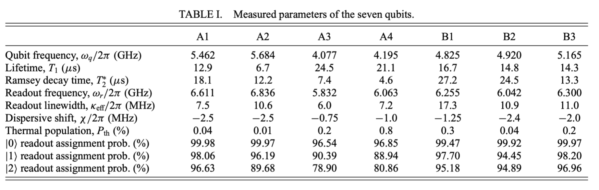

As we can see, all the qubits have very different characteristics. There’s a lot of data here, so let’s focus on the following values:
- T1 and T2—they roughly define the lifetime of a qubit. T1 defines how long does it take for the qubit to go from \(\mid 1 \rangle\) to \(\mid 0 \rangle\) and T2 measures how quickly qubit loses its phase (see section 1.1 here).
- Readout assignment probability—this basically defines the measurement error. As you can see it’s different for states \(\mid 0 \rangle\) and \(\mid 1 \rangle\) (you can disregard state \(\mid 2 \rangle\) ).
- Gate errors—the percentage values next to nodes (green) indicate one-qubit errors and next to edges the two-qubit errors (blue). This basically tells you what’s the probability that a given gate won’t do what it’s supposed to.
- Gate speed—how long it takes to execute one gate.
Ok, what does it all mean? Let’s use the most optimistic values for simplicity—lifetime of the qubit equal to 27.2\(\mu s\), gate errors 0.18% and 1.7%, and gate speed 50ns (see Fig 1c from the paper).
This means that we can apply at most \(\dfrac{24.5 \mu s}{50 ns} \approx 500\) gates to still be able to get reasonable results. What does it look like if we take gate errors into account? The probability that the result you get for a single qubit is correct is equal to (1 - gate error)^(number of gates). So if you want to be 90% sure that you got the right result, you can run 50 gates. If 80% is enough that’s about 123 gates. What about 2-qubit gates? Well, you can use only 6 of them for the 90% case and 13 for the 80% case.
To make things even worse, once you make a measurement, some of the measurements will be wrong anyway. I couldn’t find the number in this paper, but for Google’s Sycamore chip, readout error was 3.8% (see Fig 2.).
Btw. I highly recommend the paper that I took the data from, it shows you what’s the state-of-the-art implementation of QAOA on a real device. And here’s another good example from Google.
There’s also statistical uncertainty (sometimes also called “sampling noise”)—this is the error that we introduce into our estimates by the fact that we cannot directly measure the wavefunction, we need to sample from it. So having 100 measurements gives you results with more uncertainty than having 10,000 measurements. We’ll probably talk more about how to deal with that in the next article.
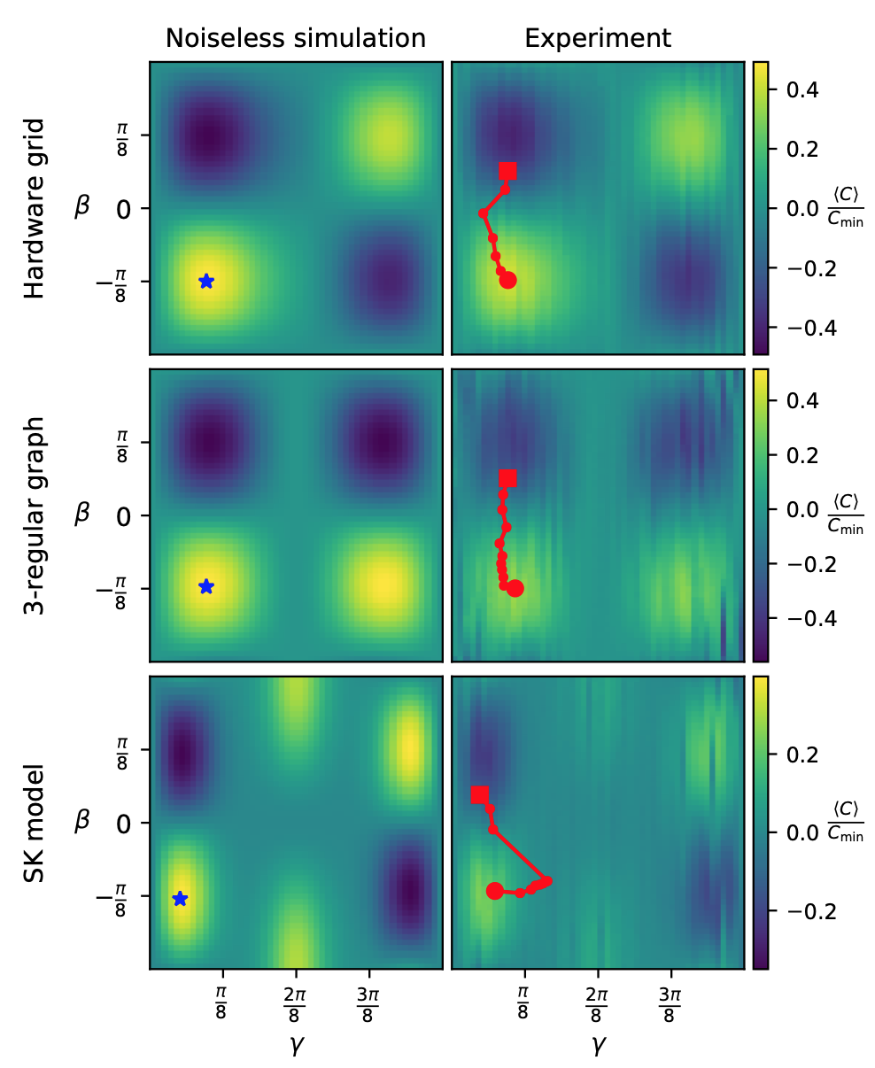
A good example of how the noise affects result are the plots of the optimization landscapes of 1 layer QAOA which came from Google’s Sycamore chip (Fig 3 in this paper):
One way to deal with these issues (at least some of them) is to use Quantum Error Correction (QEC). QEC is a set of techniques that allow you to correct some errors that can happen in your circuit. If you‘ve ever heard about the distinction between “physical” and “logical” qubits, then you might know that by “logical” people usually mean “perfect, error-corrected qubits”. Once we have such qubits, we will be in the realm of Fault-Tolerant Quantum Computing (FTQC) The problem is that in order to implement one error-corrected qubit you have to use a LOT of physical qubits (which also depends on the level and type of errors), as we encode one logical qubit in an entangled state shared by multiple physical qubits. We can design this state in such a way that the quantum information is protected against different types of noise. But since in this article we’re talking about variational algorithms and the NISQ era, we won’t actually go into this, if you’re interested check out chapter 10 from Nielsen and Chuang.
Another, quite straightforward, way to deal with some of these issues is to simply run short circuits. The fewer gates you have, the lower the chance something will go wrong. Obviously, improving the hardware also helps (or, as it turns out, improving control software responsible for gates, as shown here). But let’s get into some more algorithmic techniques.
Error mitigation
Instead of correcting the errors and getting perfect results, we can try to mitigate the errors. There are many interesting techniques (see here for a good review), here I’ll describe one of them to give you a general idea of how it can be achieved. It’s important to mention that these methods allow us to better estimate the expectation values of some operators. This means that we’ll be talking about getting certain real numbers with a specific precision, not about getting the correct set of 0s and 1s.
One of the methods is called “Zero Noise Extrapolation” (source). The main idea is that if we just run our circuit, it will be affected by a certain base level of noise. Our goal would be to know the result for the “zero noise” case, but we can’t just fix the hardware so that it doesn’t have any noise. However, we can artificially increase (scale) the level of noise. So we’ll run our circuit a couple of times, with different levels of noise, and then we’ll extrapolate it to see what happens for the “zero noise” case.
Here’s a picture that shows the idea:
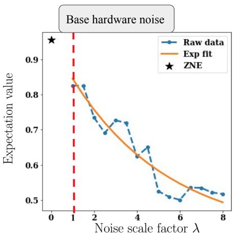
How do you artificially increase the noise? Well, there are a couple of methods to do that, one of them involves simply duplicating gates—we replace gate G by (G, G’, G), where by G’ I mean the inverse of G.
There are other error mitigation techniques, but in general, they involve running several modified versions of the original circuit and performing some post-processing to get the value we’re interested in.
If you’d like to use error mitigation techniques, there’s an open-source python library called mitiq developed by folks from Unitary Fund. You can learn more about ZNE and other methods, as well as about mitiq from this talk by Ryan LaRose (which is also the source of the plot you see above).
There’s one more important caveat here – what I described is mitigation by “classical postprocessing”. There’s another way to achieve error mitigation by performing certain actions during the execution of the circuit which counteract the noise.
Compilation
Well… If noise itself wasn’t bad enough, there are other issues which make its existence even worse. It’s the device connectivity (i.e. which qubits are directly connected, so you can use a two-qubit gate between them) and gate set (i.e. which gates you can directly execute on the hardware)1
How do you deal with these? Two basic methods are compilation and ansatz design, and in this section, we’ll talk about the first of these. To be honest—I know very little about compilation, so this section definitely doesn’t do justice to the topic, though I think it’s important to include it for the sake of completeness.
What is compilation? It’s transforming one quantum circuit into another one that does exactly the same thing.
Usually, we do compilation for the following reasons (in no particular order):
- Our circuit doesn’t map well on the hardware architecture (dealing with connectivity)
- Our circuit uses gates that are not directly implemented on the device (dealing with the native gate set)
- We want to minimize the number of gates (reducing the impact of noise). Usually, we care mostly about 2-qubit gates, as they are much more noisy than 1-qubit gates.
There are different approaches to compilation, here I present three that I’m aware of:
- Rule-based—we define a set of rules (e.g. how to decompose a gate into a set of other gates) that we then simply apply to the circuit.
- We treat circuits as some mathematical structure and perform some mathmagic to simplify it, for example using ZX calculus. Don’t ask me for any more details, I’ve personally chosen to just think about it as mathmagic (though to be honest I’ve heard this review is a decent intro to ZX calculus, I simply never got to reading it. There’s also this open source package.).
- Machine Learning—well, you can also just throw some machine learning at the problem, as they did in Harrigan et al.
If anyone is interested in the topic this article might be helpful. Another important theoretical result to mention is the Solovay-Kitaev theorem—it basically says that we can approximately compile any unitary operation into a limited set of gates quite efficiently (with some caveats, of course, more on wiki).
That’s it for now, if I learn more about the topic I’ll revisit and improve this part. Let’s now get into the topic much closer to my heart. Namely…
Optimization
Ok, we’ve covered some general, hardware-related issues. Now it’s time to talk about the more algorithmic part. One of the central components of VQAs is the optimization loop and there’s indeed a lot of research on this topic. So let’s see what are some of the main challenges involved:
Barren plateaus
Imagine you want to find the lowest point in some area. How would you do that? Well, you can just look around, follow the slope and you’ll eventually get somewhere. Doesn’t sound like the best possible strategy—if you’re in the mountains you’ll soon find some valley, though not necessarily the lowest/deepest one. But at least you’re getting somewhere. Do you know what’s a nightmare scenario in such a case?
A huge desert.
You’re not able to see anything but flat sand all the way to the horizon and the landscape constantly changes as the wind reshapes the dunes.
What’s the only chance you have of actually finding what you’re looking for? Start from a point that’s so close to the valley you’re looking for that you just can’t miss it. What’s another name for a landscape like this?
A barren plateau.
In 2018 Jarrod McClean et al. pointed out that there are two big problems with training variational quantum circuits.
The first is that you can’t just run a single circuit and learn what the value of the gradient is (we’ve discussed it in the previous VQA post). You need to repeat a certain procedure several times and the more times you do it, the better accuracy you get. This is not a big problem if your gradient is huge; let’s say it has a value of 9001. You just repeat the procedure several times and you know the ballpark. But what if your gradient has a value of 0.00001? Well, you have to run many many more circuits (for those interested—in the best case it scales as \(O(1/ \epsilon)\), where \(\epsilon\) is desired accuracy.)2
The second is, that for random quantum circuits the gradient is really small in most places except for some small area where it’s not. And the chance that it’s arbitrarily close to zero for a random point grows exponentially with the number of qubits and number of parameters (see this PennyLane tutorial for more context).
Ok, now let’s put it together in plain English. In most places, the gradient is close to 0 and from the practical perspective, there’s a limit to the precision up to which you can estimate it. So basically unless you start close to good parameters, you have no clue how to tweak your parameters to get anything reasonable. And the more qubits or gates you have, the worse it gets.
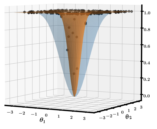
I also like the plot below (source: Cerezo et al.) which visualizes the problem. It shows how the landscape changes when we increase number of variables in the cost function (from 4 (blue) to 24 (orange)).
As a side note, I find this problem shows quite well one of the problems with the state of quantum computing research. As long as you’re running small simulations, this effect is too small to be noticed. So some previous small experiments might be fundamentally flawed because if you tried to scale them up, you would hit the barren plateau problem. On the other hand, there might be other problems that we’ll notice only when we’ll get to hundreds of qubits. These are exciting times to be working on QC!
Dealing with barren plateaus
Not surprisingly, these findings resulted in quite some stir in the community. People started coming up with various methods to solve this issue and here we’ll go through a couple of them. Let’s look at the two common approaches for dealing with this problem.
The first way is to simply initialize your parameters close enough to the minimum so that your optimizer can find its way to the minimum. This might sound like a no-brainer—sure we want to have a good way of initializing the parameters, right? Actually, it’s not that obvious, as in classical machine learning, it usually is not that big of a problem and you can get away with initializing parameters randomly. So how do you choose a reasonable parameter initialization? There are several methods to do that, one of them is the so-called “layer by layer” (LBL) training3
Many ansatzes we use consist of layers. Basically, all the layers are identical and (at least in theory), the more layers you add, the more powerful your circuit is (QAOA is a good example). So here the idea is that we start from training our algorithm for one layer. Since barren plateaus depend on both the number of qubits and the depth of the circuit, it should allow us to avoid them. Then, once the 1st layer is optimized, we treat it as fixed and train parameters for the second layer. Once its training is finished, we proceed with the next one until we have all the layers we wanted. Now we have some initial guesses of the parameters and we proceed to train more than one layer at a time e.g. 25% of them.
So at first, we try to avoid barren plateaus by training only a handful of parameters at the time. And then, we try to avoid them by starting from a point that is already a pretty good guess.
The second idea is about restricting the parameter space—if you can design your ansatz specifically for a given problem, it might be less expressible (we’ll talk about expressibility in a moment), but as long as it can find the solution to your problem, it doesn’t really matter.
Just to put things in perspective, since the initial paper published in March 2018, I’ve counted 18 papers with the words “barren plateaus” in the title and the phrase was cited 263 times according to Google Scholar. If this problem sounds interesting to you, some good papers to read would be those about what are the sources plateaus (entanglement and noise), or some mathematical ways to avoid them.
Choice of optimization methods
A question that I sometimes hear is “are there optimizers that are specific for quantum computing”? In principle no, as you can treat the calculation of the cost function in the variational loop as a black box, and therefore you can use any optimization method for that. However, there are certain challenges associated with our particular black box that might make some optimizers a much better fit than the others.
So the first challenge is that in general, we consider the time spent running algorithms on a quantum chip much more expensive (money-wise) than on a classical one. Therefore, since we use it exclusively for calculating the value of the cost function, evaluating the cost function is the most expensive part of the algorithm. Thus, it is something we want to do as little as we can get away with (isn’t it somewhat ironic, that when we run calculations of a quantum computer, we want to use it as little as possible?). The practical meaning of this is that we want to use optimizers that can work well while making a relatively small number of evaluations.
The second challenge is the probabilistic nature of the cost function evaluation. In order to deal with it, you need to repeat your circuit more times to have better accuracy. Or using an optimizer, which works well with some level of noise/uncertainty.
The third challenge is the existence of noise. Noise might have different effects on the landscape of the cost function. One is “flattening of the landscape,” another might be the existence of some artifacts. Both these effects are visible in the plot we’ve QAOA landscapes we’ve seen before.
Last, but not least, it’s extremely hard to study the behavior of the optimizers. They often rely on hyperparameters (e.g.: step size in gradient descent), their behavior might be different for different problems. This is a problem not only for QC, this is the same for classical optimization problems or regular Machine Learning. Also, the cost of implementing and checking the performance of various optimizers is really high, so researchers usually either decide to use one that worked for them in the past or one that is commonly used or perhaps check a couple of them and pick the one that looks reasonable. Yet another issue is that sometimes these methods are studied without the noise (where they work well), but they don’t perform that well in the presence of noise.
My plan was to follow this section with a selection of some widely used optimizers, and explanations why some of them are widely used. But after digging into the literature, I wasn’t able to come up with anything satisfactory. It basically looks that right now we have little to no idea why certain optimizers work while others don’t. So if you’re interested in this topic, I recommend the following papers: Sung et al. and Lavrijsen et al.. Excellent work which shows how hard it is to analyze these and how much we still need to learn.
Ansatz design
We’ve already mentioned ansatzes in the previous section, but let’s now make them our main focus. Ansatz design is an active field of research, some of my favorite papers are those by Sukin Sim and other folks from Zapata, Lena Funcke et al. and J. Lee et al.. Since I like to be practical, let’s look at this from a practical perspective:
- How can you tell whether an ansatz is a good one?
- How to design a good ansatz?
Is my ansatz any good?
In the NISQ world, when you have an ansatz, you want to ask yourself two questions:
- How powerful is my ansatz?
- How much does it cost to use it?
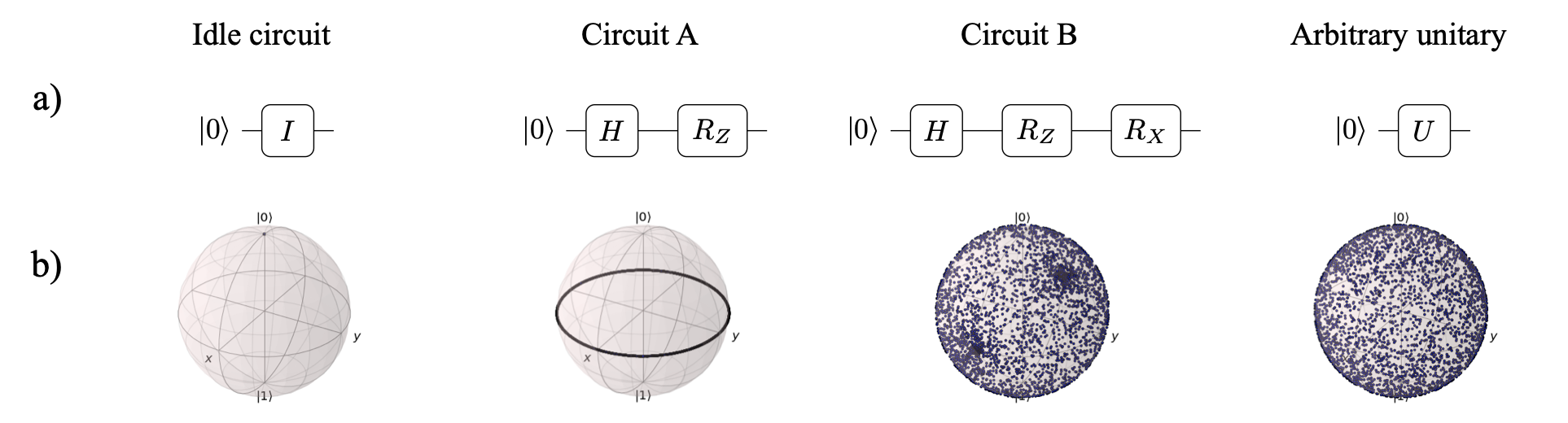
What does powerful mean in this context? One component is its expressibility—i.e. whether we can create an arbitrary state with it. The best illustration of this concept I know is the picture below (source Sim et al.). It shows how changing the circuit changes the amount of the space that we can cover.
Another useful metric is the entangling capability of an ansatz. We want the ansatz to be able to produce highly entangled states, as the more entanglement there is, the more “quantum” it is and potentially more useful.
These metrics are the best we have, but unfortunately, they are not really very good. Expressibility might not be a good metric for large circuits as more expressive circuits might be also more prone to barren plateaus or have more parameters and be harder to optimize. Entangling capability—well, creating circuits that are hard to simulate just for its own sake doesn’t make much sense.
Therefore, we can use these two metrics as something that can help us rule out bad ansatzes, but not necessarily find the best ones. Some further reading: Haug et al. and Cerezo et al.
When it comes to cost, typical metrics to measure the cost are:
- Circuit depth—the more shallow the circuit, the better chance that noise won’t destroy our quantum state.
- Circuit connectivity—since on many NISQ devices we cannot directly connect arbitrary qubits, it might be beneficial to have an ansatz which only requires connectivity between nearest neighbors.4
- Number of parameters—fewer parameters mean an easier job for optimization.5
- Number of two-qubit gates—usually two-qubit gates are much more noisy than one-qubit gates, so this number is often used to compare different circuits.
- Gate types—it’s a little bit more indirect, but if we have an ansatz which uses gates that are not available on our hardware, we will need to decompose gates, which increases circuit depth.
How to design a good ansatz
Now we want to have an ansatz for which expressibility and entangling capabilities are high, while we keep all the associated costs to a minimum, right?
Easier said than done :) How do you come up with the idea for the ansatz in the first place? At the moment there are two main schools: problem-motivated and hardware-motivated ansatz design.
To design a problem-motivated ansatz, you do things like:
- Thinking hard about the problem you want to solve
- Analyzing whether there is any structure in the problem you can exploit
- Reading existing literature on “classical” (meaning not QC) methods for solving this problem to get inspired.
To design a hardware-motivated ansatz, you do things like:
- Memorizing technical specs of the device you have
- Figuring out how to make maximally expressive ansatz given the hardware constraints
- Reading existing literature on this type of hardware to find some tricks you can exploit or traps you can fall into.
As always, both methods have some pros and cons that I’ve summarized below, and combining both of them probably is the best solution.
Problem-motivated
Pros:
- Can exploit problem structure
- Can be used with different devices
- Doesn’t require intricate knowledge about the hardware
Cons:
- Might not be implementable on specific hardware
- Might perform poor on real hardware while working perfectly in theory
- Probably will work only for a narrow class of problems
Hardware-motivated
Pros:
- Allows to squeeze the most out of the device
- Doesn’t require intricate knowledge about the problem domain
- Can be used for solving multiple problems
Cons:
- Might not take advantage of the problem’s structure
- Is probably useful only for a very specific device
One consequence of coming from the problem-focused approach is that you don’t necessarily want to have the maximally expressible ansatz. While such an ansatz would by definition cover your solution, it will also cover all the solutions that you might a priori know are useless. Often we have some knowledge about the problem and we know that a certain family of states does not contain the ground state, so we can make our ansatz simpler (and hence lower the cost) by designing it in a way that excludes such states.
How to get a good ansatz without designing it?
There’s yet another method for finding a good ansatz—let the algorithm figure it out. To do that, we use what are called “adaptive” algorithms. The main idea is that we modify not only the parameters of the circuit, but also the structure of the circuit itself during the optimization.
One example of such a method and the first such algorithm proposed is a method called ADAPT-VQE. Here’s a general description of how it works:
- Define an “operator pool”—this basically contains the bricks that you’ll be building your algorithm from.
- Create some initial reference state as the first iteration of your ansatz.
- Calculate the gradient of the expectation value for each operator in the pool using your ansatz.
- Add the operator with the biggest gradient to the ansatz (along with a new variational parameter).
- Run “regular VQE” with this ansatz to optimize all the parameters of the ansatz.
- Go to step 3.
For a more detailed description please see Grimsley et al.).
Another example of an adaptive method is PECT, which I have mentioned in the previous article .
Here are some comments about these methods:
- These algorithms are usually more difficult to implement on the classical side, as they involve more than just taking a parametrized circuit and adjusting the parameters, but also changing its structure.
- It’s not obvious whether such an approach actually yields better results or produces them faster. There are two effects that are at play—on one hand, the algorithm should need more time than a conventional one because it needs to find the correct structure of the ansatz and optimize its parameters at the same time (in point 5 of ADAPT-VQE we’re running a full, regular VQE!). On the other hand, doing both at the same time makes the optimization process actually simpler as it doesn’t introduce (or gets rid of) parameters that are useless. In principle it should find better solutions, however, it might take longer—it’s hard to say before actually running it for a specific problem.
- These algorithms seem especially promising for NISQ devices, as they produce ansatzes that are shallower than those designed by hand (and hence there’s less room for noise), but also they naturally find circuits that take into account all the quirks of a specific device. For example, in ADAPT-VQE you can create an operator pool in such a way that it leads to hardware-efficient ansatzes (see Tang et al. ).
If you want to learn more about ADAPT-VQE and the problem of ansatz design in general, Sophia Economou (one of the authors of ADAPT-VQE) gave an excellent 25-minute talk about these during one of Quantum Research Seminar Toronto (QRST).
As a side note, this approach reminds me of a NEAT (Neuroevolution of Augmenting Topologies) algorithm used for classical neural networks. You can find an excellent video showing how a NEAT algorithm learns to play Mario.
Interpolating algorithms
The approach which makes me particularly excited is something I’ll call “interpolating algorithms.”6 What do we mean by “interpolating”? The fact that the performance of these algorithms can interpolate between that of near-term and far-term algorithms. You can adjust some hyperparameters of the algorithm depending on what hardware you’re running on, so no matter what stage of development of quantum hardware we’re currently at (from now to perfect qubits), you can find hyperparameters that will allow you to actually run the algorithm within the limitations of the hardware and squeeze most out of it.
Imagine you have circuit A that allows you to estimate the ground state of some Hamiltonian. If you want to estimate it to precision \(\epsilon\), you would need to run circuit A \(N_A=\frac{1}{\epsilon^2}\) times. You also have circuit B, that allows you to get the same precision, but you only need to run it \(N_B = log(\frac{1}{\epsilon})\) times. However, circuit B is \(\frac{1}{\epsilon}\) times longer and hence not very practical for the devices we have today. But what if we had some way to interpolate between these two approaches so that we would have a parameter that makes the circuit longer, but also decreases the number of samples needed?
Let’s see what it could look like in practice. Let’s say \(\epsilon=10^{-3}\). This means we need to run circuit A 1,000,000 times and each execution of circuit A takes 1ms. So the total runtime will be 1,000s. For circuit B we need to run it log(1000) times, which is just 3 times (sic!), though each execution takes 1 second. Hence we would get our result in just 3 seconds. Unfortunately, as we have seen earlier, our circuit probably won’t be able to run for as long as 1 second anytime soon. However, this class of algorithms gives us a way to construct such a circuit that it requires less measurements but its execution time still fits our hardware.
While this explanation is oversimplified , going into more details is, again, way beyond the scope of this article. If you’d like to learn more, three examples of similar approach are “alpha-VQE”, “Power Law Amplitude Estimation” and “Bayesian Inference with Engineered Likelihood Functions for Robust Amplitude Estimation” by my colleagues from Zapata . (I strongly recommend watching this 3.5-minute video explaining the gist of it).
Other issues
This article has been quite dense, so here I wanted to just point to some other final issues that are prevalent in contemporary research, without spending too much time on any of them:
Lack of common benchmarks and standardization
As you could see from the section about optimizers, it’s really hard to benchmark certain solutions. It’s not only extremely costly to compare multiple methods, but it’s also really hard to design such an experiment in a way that makes the comparison fair and broadly useful.
On top of that, as can be expected for a discipline at such an early stage, we lack standardization. This is healthy, as it allows for more experimentation and exploration, but it makes it much harder to compare results, as you basically never compare apples to apples.
We have no idea what we’re doing
The truth is that QC is a totally new paradigm of computation that we don’t comprehend. I‘ve had the opportunity to talk with some excellent researchers in the field and while their level of understanding and intuition about these matters is far beyond my reach, they’re quite open about the fact that we all just started scratching the surface. There are some fundamental questions that no one knows the answers to, which is both a challenge and a source of excitement.
Scaling for bigger devices
In most of our research, we’re limited in what we can analyze by the size of the devices we’re able to simulate with computers (rarely beyond 30 qubits). Bigger devices are extremely scarce—there is literally a handful of them in the world—so we have very little understanding of how these methods will scale beyond 50 qubits. And while some results seem independent of size or we have some theory that explains how they will behave, for many we don’t. And right now there’s no other way of knowing other than building bigger devices and trying them out.
Closing notes
Thank you for going through this whole article! If this was of interest for you, you’ll definitely like the next part, where I focused on VQE. The best way not to miss any future articles is to subscribe to the newsletter.
So just in case you have missed them, I recommend checking out:
- My podcast.
- QOSF monthly challenges—especially if you’d like to hone both your coding skills and learn some interesting QC concepts.
Last, but not least, I wanted to thank all the people that helped me write this article. And this time that was more people than usually:
- Pierre-Luc Dallaire-Demers for being an infinite well of knowledge and references. His help reduces the complexity of looking for references from \(O(n)\) (searching through \(n\) papers) to \(O(1)\) (asking one Pierre-Luc).
- Rafał Ociepa for all editing and stylechecks.
- Alba Cervera-Lierta, Ntwali Bashige and Peter Johnson for reviewing the whole thing with their eagle eyes and making sure I’m not saying something stupid.
- Ahmed Darwish and Alex Juda also for reviewing the whole thing and being my test “target audience”.
- Sophia Economou and Sukin Sim for reviewing specific sections associated with their research.
Have a nice day!
Michał
Footnotes:
-
For explanation why these are problematic please see VQA blogpost. ↩
-
Numbers here are totally fake, I’m just making a point. ↩
-
Another example: E. Grant et al. ↩
-
This depends on the hardware type, as it’s a much bigger issue for superconducting qubits rather than ion traps. ↩
-
Though there are some counterarguments, see Kim et al or Lee et al. ↩
-
There’s no proper name for this class of algorithms in the literature yet. ↩